Animations

An animation is "something" that changes in time. This something can be a simple double, an Angle, a Point3D, …

Let us consider the most basic of animations: the double animation that goes from 0 to 1 in 1 second. If we are to visualize this, we would get:

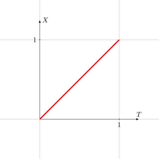
The animation is actually a function mapping time values to double values. Let’s denote this function with \(X(t)\). We can translate the properties above to mathematical formulae: in the very beginning, the animated double should have value \(0\). This is expressed by

Next, we know the animation takes 1 second to finish and that the double should have value \(1\) at that time:

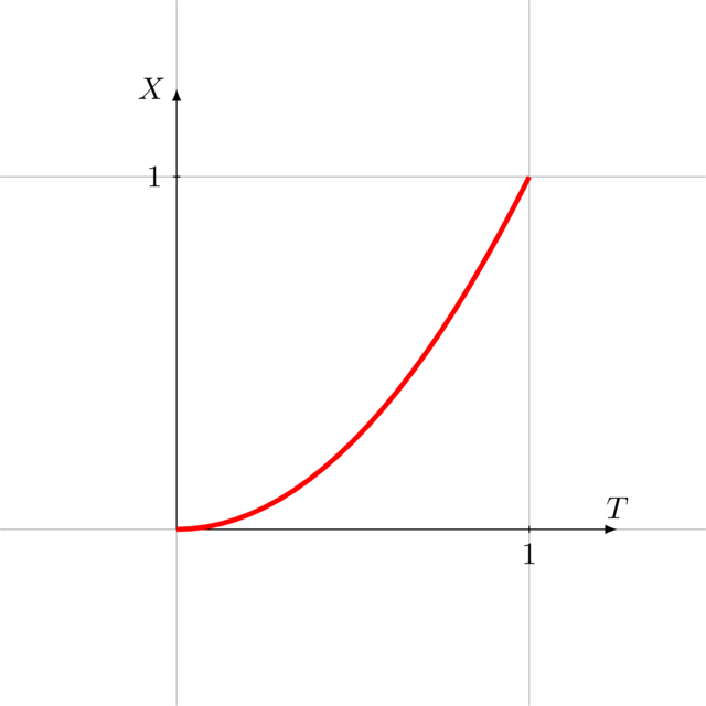
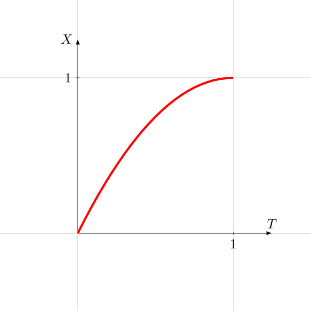
Now, there are many ways in which we could want to modify this animation. For example, we assumed that the double moves "in a straight line" from 0 to 1. Other possibilities would be

We may also want to change the starting and ending value of the animation, e.g. have a double go from 10 to 20. The duration is also an aspect we may wish to modify.

While we could bundle all parameters together into one 'superanimation', we prefer to keep things modular.

Before modifying the basic animation, let’s first focus on the mathematical formula behind it.

We know the animation goes in a straight line, meaning \(X(t)\) has the form \(m \cdot t + q\) where \(m\) and \(q\) can be deduced from the constraints \(X(0) = 0\) and \(X(1) = 1\). We get

which is a pretty simple formula.

Say we don’t want to animate from 0 to 1, but from 10 to 20, or better, from \(a\) to \(b\). We can achieve this easily by mapping the interval \([0, 1\)] to \([a, b\)].

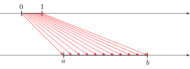
We build another function, \(f\), that can do this for us. Again this is linear function:

which gives

How can we combine this function \(f\) with the basic animation \(X(t)\) to produce an animation from \(a\) to \(b\)? Simple: we first animate \(0\) to \(1\) and use \(f\) to map the value to \( [a, b\) ]. Let’s call this new animation \(X_2(t)\).

The basic animation takes one second to complete. What if we want a shorter or longer animation?

Say we want the animation to take \(\tau\) seconds. Our time will then vary from \(0\) to \(\tau\), whereas the basic animation expects it to vary from \(0\) to \(1\). We somehow need to translate "our time" to the "basic animation’s time". Again we can do this with a linear transformation:

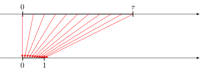
Let’s assign the name \(g\) to the function that maps the interval \([0, \tau\)] to \([0,1\)].

Given our basic animation \(X(t)\), which moves from \(0\) to \(1\) in 1 second, we can transform it to an animation \(X_3(t)\) that goes from \(0\) to \(1\) in \(\tau\) seconds as follows:

The basic animation is linear: it moves from \(0\) to \(1\) at constant speed. However, if we were to chain animations, the transition from one animation to the next would be perceived as very abrupt. Compare the animations below:

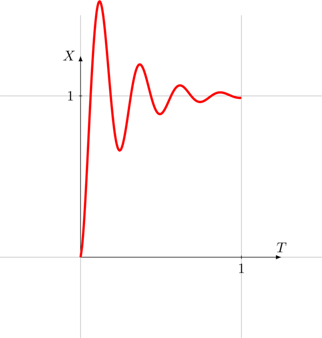
Animations can be made smoother using easing functions. Below are a few examples:

An easing function \(e(x)\) is a function for which

How it moves from \(0\) to \(1\) is up to the easing function.

If we want to apply some easing function \(e(x)\) to the basic animation \(X(t)\) yielding the new animation \(X_3(t)\), we use the following formula:

Using the range mapper \(f\), the domain mapper \(g\) and the easing function \(e\) we can transform the basic animation any way we want:

We can build a library of range mappers, domain mappers and easing functions and use them to produce any animation we want.

The double animation is the basic building block for all animations: all other animations can be built from it. Let’s introduce a convenient notation to denote double animations:

represents a double animation from \(x\) to \(y\) in \(\tau\) seconds. We ignore the shape of the animation for now, i.e. we disregard easing functions.

Say we now want to create Point3D animation \(P(t)\): we wish a movement from \((0, 0, 10)\) to \((0, 5, 0)\). The animation of a Point3D is the animation of its components, i.e. its x, y and z-coordinates:

or, more generally,

We can animate colors or any other type of value the same way: