Perlin Noise

' '

1. Deterministic Continuous Random Functions</h1>

To procedurally generate textures, we generally need a source of randomness. Libraries often offer this functionality in the form of a function that returns a new value each time it’s called.

A problem with these random number generators is that they are "too random" for our purposes. Consider the graphs below:

chaotic terrain

smooth terrain

Perlin noise is in essence a random number generator that guarantees a certain smoothness. Concretely, what we want is some function double random(double x) that satisfies the following conditions:

random must be deterministic: random(x) must return the same result when given the same x.
random must be continuous: random(x) and random(x + 0.00001) should be close to each other, i.e. no sudden jumps.

Perlin noise satisfies these criteria.

The function double random(double x) is one-dimensional: it associates a value with each double. We can lift this to higher dimensions:

double random(const Point2D&) is a two dimensional variant: it associates a value with each Point2D.
double random(const Point3D&) is three dimensional: each point in 3D space is mapped to a value.

2. Perlin Noise

Perlin noise is such a deterministic continuous function. For the remainder of this page, we will work in 2D, i.e. we will build a function double perlin(const Point2D&).

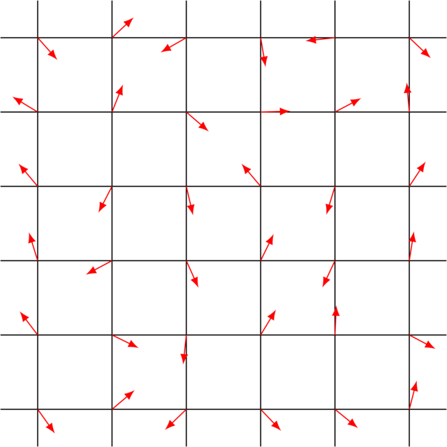
Perlin noise works as follows: take a 2D grid of 1 × 1 cells and associate a unit vector with every intersection.

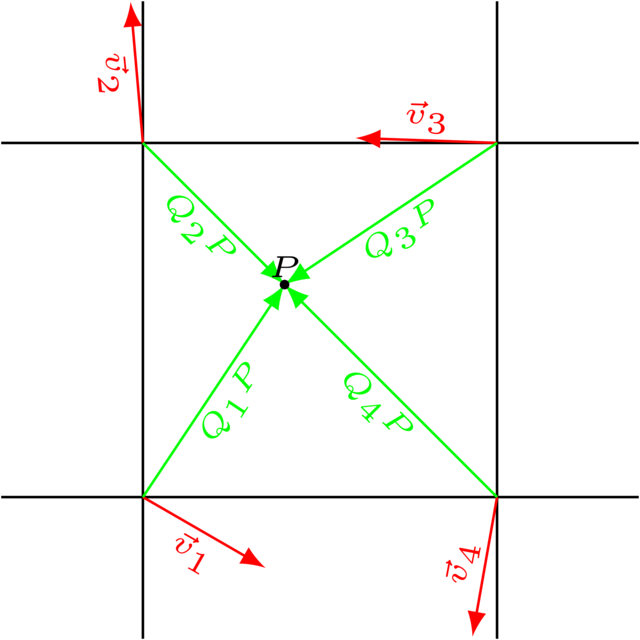
In order to determine the value associated with a point $P(x, y)$ , you need to find out in which grid cell it resides. Its corners are

$Q_1(\lfloor x \rfloor, \lfloor y \rfloor) \qquad Q_2(\lfloor x \rfloor, \lceil y \rceil) \qquad Q_3(\lceil x \rceil, \lceil y \rceil) \qquad Q_4(\lceil x \rceil, \lfloor y \rfloor) \qquad$

where $\lfloor x \rfloor$ corresponds to rounding $x$ down and $\lceil x \rceil$ to rounding $x$ up. Each corner has a unit vector associated with it. We denote the vector corresponding to $Q_i$ with $\vec v_i$ .</p>

Next, take the dot product of each $Q_iP$ and $v_i$ :

$z_i = (P - Q_i) \cdot v_i$

Now we have associated a $z$ -value with each corner. As last step, we need to determine which $z$ -value to assign to $P$ itself using interpolation.

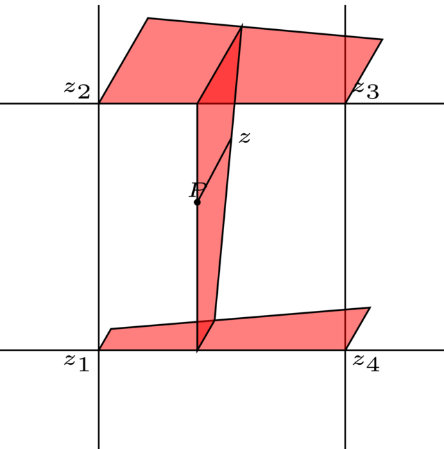
Interpolation goes in three steps:

Find a function $f$ with $f(0) = z_1$ and $f(1) = z_4$ . Compute $f(x)$ .
Find a function $g$ with $g(0) = z_2$ and $g(1) = z_3$ . Compute $g(x)$ .
Find a function $h$ with $h(0) = f(x)$ and $h(1) = g(x)$ . Compute $h(y)$ .

The functions $f$ , $g$ and $h$ can be linear or, for better results, an easing functions.